Spectral fitting example (GRB)
To run this, you need the following files, which can be downloaded using the first few cells of this notebook:
orientation file (20280301_3_month_with_orbital_info.ori)
binned data (grb_bkg_binned_data.hdf5, grb_binned_data.hdf5, & bkg_binned_data_1s_local.hdf5)
detector response (SMEXv12.Continuum.HEALPixO3_10bins_log_flat.binnedimaging.imagingresponse.nonsparse_nside8.area.good_chunks_unzip.h5.zip)
The binned data are simulations of GRB090206620 and albedo photon background produced using the COSI SMEX mass model. The detector response needs to be unzipped before running the notebook.
This notebook fits the spectrum of a GRB simulated using MEGAlib and combined with background.
3ML is a high-level interface that allows multiple datasets from different instruments to be used coherently to fit the parameters of source model. A source model typically consists of a list of sources with parametrized spectral shapes, sky locations and, for extended sources, shape. Polarization is also possible. A “coherent” analysis, in this context, means that the source model parameters are fitted using all available datasets simultanously, rather than performing individual fits and finding a well-suited common model a posteriori.
In order for a dataset to be included in 3ML, each instrument needs to provide a “plugin”. Each plugin is responsible for reading the data, convolving the source model (provided by 3ML) with the instrument response, and returning a likelihood. In our case, we’ll compute a binned Poisson likelihood:
where \(d_i\) are the counts on each bin and \(\lambda_i\) are the expected counts given a source model with parameters \(\mathbf{x}\).
In this example, we will fit a single point source with a known location. We’ll assume the background is known and fixed up to a scaling factor. Finally, we will fit a Band function:
where \(K\) (normalization), \(\alpha\) & \(\beta\) (spectral indeces), and \(x_p\) (peak energy) are the free parameters, while \(E_{piv}\) is the pivot energy which is fixed (and arbitrary).
Considering these assumptions:
where \(B*b_i\) are the estimated counts due to background in each bin of the Compton data space with \(B\) the amplitude and \(b_i\) the shape of the background, and \(s_i\) are the corresponding expected counts from the source, the goal is then to find the values of \(\mathbf{x} = [K, \alpha, \beta, x_p]\) and \(B\) that maximize \(\mathcal{L}\). These are the best estimations of the parameters.
The final module needs to also fit the time-dependent background, handle multiple point-like and extended sources, as well as all the spectral models supported by 3ML. Eventually, it will also fit the polarization angle. However, this simple example already contains all the necessary pieces to do a fit.
[1]:
from cosipy import COSILike, BinnedData
from cosipy.spacecraftfile import SpacecraftFile
from cosipy.response.FullDetectorResponse import FullDetectorResponse
from cosipy.util import fetch_wasabi_file

from scoords import SpacecraftFrame

from astropy.time import Time
import astropy.units as u
from astropy.coordinates import SkyCoord
from astropy.stats import poisson_conf_interval

import numpy as np
import matplotlib.pyplot as plt
%matplotlib inline

from threeML import Band, PointSource, Model, JointLikelihood, DataList
from cosipy import Band_Eflux
from astromodels import Parameter

from pathlib import Path

import os
08:46:50 WARNING   The naima package is not available. Models that depend on it will not be         functions.py:48
                  available
         WARNING   The GSL library or the pygsl wrapper cannot be loaded. Models that depend on it  functions.py:69
                  will not be available.
08:46:53 WARNING   The ebltable package is not available. Models that depend on it will not be     absorption.py:33
                  available
08:46:54 INFO Starting 3ML! __init__.py:39
WARNING WARNINGs here are NOT errors __init__.py:40
WARNING but are inform you about optional packages that can be installed __init__.py:41
WARNING to disable these messages, turn off start_warning in your config file __init__.py:44
WARNING no display variable set. using backend for graphics without display (agg) __init__.py:50
08:46:55 WARNING ROOT minimizer not available minimization.py:1345
WARNING Multinest minimizer not available minimization.py:1357
WARNING PyGMO is not available minimization.py:1369
08:46:56 WARNING   The cthreeML package is not installed. You will not be able to use plugins which  __init__.py:94
                  require the C/C++ interface (currently HAWC)
         WARNING   Could not import plugin FermiLATLike.py. Do you have the relative instrument     __init__.py:144
                  software installed and configured?
         WARNING   Could not import plugin HAWCLike.py. Do you have the relative instrument         __init__.py:144
                  software installed and configured?
08:47:00 WARNING No fermitools installed lat_transient_builder.py:44
08:47:00 WARNING   Env. variable OMP_NUM_THREADS is not set. Please set it to 1 for optimal         __init__.py:387
                  performances in 3ML
         WARNING   Env. variable MKL_NUM_THREADS is not set. Please set it to 1 for optimal         __init__.py:387
                  performances in 3ML
         WARNING   Env. variable NUMEXPR_NUM_THREADS is not set. Please set it to 1 for optimal     __init__.py:387
                  performances in 3ML
Download and read in binned data
Define the path to the directory containing the data, detector response, orientation file, and yaml files if they have already been downloaded, or the directory to download the files into
[4]:
data_path = Path("/path/to/files")
Download the orientation file (684.38 MB)
[6]:
fetch_wasabi_file('COSI-SMEX/DC2/Data/Orientation/20280301_3_month_with_orbital_info.ori', output=str(data_path / '20280301_3_month_with_orbital_info.ori'))
Download the binned GRB+background data (75.73 KB)
[8]:
fetch_wasabi_file('COSI-SMEX/cosipy_tutorials/grb_spectral_fit_local_frame/grb_bkg_binned_data.hdf5', output=str(data_path / 'grb_bkg_binned_data.hdf5'))
Download the binned GRB data (76.90 KB)
[19]:
fetch_wasabi_file('COSI-SMEX/cosipy_tutorials/grb_spectral_fit_local_frame/grb_binned_data.hdf5', output=str(data_path / 'grb_binned_data.hdf5'))
Download the binned background data (255.97 MB)
[20]:
fetch_wasabi_file('COSI-SMEX/cosipy_tutorials/grb_spectral_fit_local_frame/bkg_binned_data_1s_local.hdf5', output=str(data_path / 'bkg_binned_data_1s_local.hdf5'))
Download the response file (839.62 MB). This needs to be unzipped before running the rest of the notebook
[17]:
fetch_wasabi_file('COSI-SMEX/DC2/Responses/SMEXv12.Continuum.HEALPixO3_10bins_log_flat.binnedimaging.imagingresponse.nonsparse_nside8.area.good_chunks_unzip.h5.zip', output=str(data_path / 'SMEXv12.Continuum.HEALPixO3_10bins_log_flat.binnedimaging.imagingresponse.nonsparse_nside8.area.good_chunks_unzip.h5.zip'))
Read in the spacecraft orientation file & select the beginning and end times of the GRB
[5]:
ori = SpacecraftFile.parse_from_file(data_path / "20280301_3_month_with_orbital_info.ori")
tmin = Time(1842597410.0,format = 'unix')
tmax = Time(1842597450.0,format = 'unix')
sc_orientation = ori.source_interval(tmin, tmax)
Create BinnedData objects for the GRB only, GRB+background, and background only. The GRB only simulation is not used for the spectral fit, but can be used to compare the fitted spectrum to the source simulation
[6]:
grb = BinnedData(data_path / "grb.yaml")
grb_bkg = BinnedData(data_path / "grb.yaml")
bkg = BinnedData(data_path / "background.yaml")
Load binned .hdf5 files
[7]:
grb.load_binned_data_from_hdf5(binned_data=data_path / "grb_binned_data.hdf5")
grb_bkg.load_binned_data_from_hdf5(binned_data=data_path / "grb_bkg_binned_data.hdf5")
bkg.load_binned_data_from_hdf5(binned_data=data_path / "bkg_binned_data_1s_local.hdf5")
Define the path to the detector response
[8]:
dr = str(data_path / "SMEXv12.Continuum.HEALPixO3_10bins_log_flat.binnedimaging.imagingresponse.nonsparse_nside8.area.good_chunks_unzip.h5") # path to detector response
Perform spectral fit
Define time window of binned background simulation to use for background model
[9]:
bkg_tmin = 1842597310.0
bkg_tmax = 1842597550.0
bkg_min = np.where(bkg.binned_data.axes['Time'].edges.value == bkg_tmin)[0][0]
bkg_max = np.where(bkg.binned_data.axes['Time'].edges.value == bkg_tmax)[0][0]
Set background parameter, which is used to fit the amplitude of the background, and instantiate the COSI 3ML plugin
[10]:
bkg_par = Parameter("background_cosi",                                                                          # background parameter
                    0.1,                                                                                        # initial value of parameter
                    min_value=0,                                                                                # minimum value of parameter
                    max_value=5,                                                                                # maximum value of parameter
                    delta=1e-3,                                                                                 # initial step used by fitting engine
                    desc="Background parameter for cosi")

cosi = COSILike("cosi",                                                                                         # COSI 3ML plugin
                dr = dr,                                                                                        # detector response
                data = grb_bkg.binned_data.project('Em', 'Phi', 'PsiChi'),                                      # data (source+background)
                bkg = bkg.binned_data.slice[{'Time':slice(bkg_min,bkg_max)}].project('Em', 'Phi', 'PsiChi'),    # background model
                sc_orientation = sc_orientation,                                                                # spacecraft orientation
                nuisance_param = bkg_par)                                                                       # background parameter
Define a point source at the known location with a Band function spectrum and add it to the model
[11]:
l = 93.
b = -53.

alpha = -1                                       # Setting parameters to something reasonable helps the fitting to converge\n",
beta = -3
xp = 450. * u.keV
piv = 500. * u.keV
K = 1 / u.cm / u.cm / u.s / u.keV

spectrum = Band()

spectrum.beta.min_value = -15.0

spectrum.alpha.value = alpha
spectrum.beta.value = beta
spectrum.xp.value = xp.value
spectrum.K.value = K.value
spectrum.piv.value = piv.value

spectrum.xp.unit = xp.unit
spectrum.K.unit = K.unit
spectrum.piv.unit = piv.unit

source = PointSource("source",                     # Name of source (arbitrary, but needs to be unique)
                     l = l,                        # Longitude (deg)
                     b = b,                        # Latitude (deg)
                     spectral_shape = spectrum)    # Spectral model

# Optional: free the position parameters
#source.position.l.free = True
#source.position.b.free = True

model = Model(source)                              # Model with single source. If we had multiple sources, we would do Model(source1, source2, ...)

# Optional: if you want to call get_log_like manually, then you also need to set the model manually
# 3ML does this internally during the fit though
cosi.set_model(model)
Gather all plugins and combine with the model in a JointLikelihood object, then perform maximum likelihood fit
[12]:
plugins = DataList(cosi) # If we had multiple instruments, we would do e.g. DataList(cosi, lat, hawc, ...)

like = JointLikelihood(model, plugins, verbose = False)

like.fit()
08:49:04 INFO set the minimizer to minuit joint_likelihood.py:1045
Adding 1e-12 to each bin of the expectation to avoid log-likelihood = -inf.
08:49:30 WARNING   get_number_of_data_points not implemented, values for statistical        plugin_prototype.py:130
                  measurements such as AIC or BIC are unreliable
Best fit values:
| result | unit | |
|---|---|---|
| parameter | ||
| source.spectrum.main.Band.K | (3.10 -0.20 +0.21) x 10^-2 | 1 / (keV s cm2) |
| source.spectrum.main.Band.alpha | (-2.8 +/- 0.5) x 10^-1 | |
| source.spectrum.main.Band.xp | (4.75 +/- 0.05) x 10^2 | keV |
| source.spectrum.main.Band.beta | -6.8 +/- 1.2 | |
| background_cosi | (1.65 +/- 0.13) x 10^-1 |
Correlation matrix:
| 1.00 | 0.97 | -0.37 | 0.20 | -0.00 |
| 0.97 | 1.00 | -0.16 | 0.17 | -0.00 |
| -0.37 | -0.16 | 1.00 | -0.17 | -0.02 |
| 0.20 | 0.17 | -0.17 | 1.00 | 0.00 |
| -0.00 | -0.00 | -0.02 | 0.00 | 1.00 |
Values of -log(likelihood) at the minimum:
| -log(likelihood) | |
|---|---|
| cosi | 42920.049338 |
| total | 42920.049338 |
Values of statistical measures:
| statistical measures | |
|---|---|
| AIC | 85838.098676 |
| BIC | 85840.098676 |
[12]:
(                                      value  negative_error  positive_error  \
 source.spectrum.main.Band.K        0.030997       -0.002034        0.002123
 source.spectrum.main.Band.alpha   -0.276547       -0.052063        0.049971
 source.spectrum.main.Band.xp     474.654036       -4.933778        4.828668
 source.spectrum.main.Band.beta    -6.755004       -1.205494        1.231109
 background_cosi                    0.164940       -0.012464        0.012279

                                     error             unit
 source.spectrum.main.Band.K      0.002079  1 / (keV s cm2)
 source.spectrum.main.Band.alpha  0.051017
 source.spectrum.main.Band.xp     4.881223              keV
 source.spectrum.main.Band.beta   1.218301
 background_cosi                  0.012371                   ,
        -log(likelihood)
 cosi       42920.049338
 total      42920.049338)
Error propagation and plotting
Define Band function spectrum injected into MEGAlib
[13]:
alpha_inj = -0.360
beta_inj = -11.921
E0_inj = 288.016 * u.keV
xp_inj = E0_inj * (alpha_inj + 2)
piv_inj = 1. * u.keV
K_inj = 0.283 / u.cm / u.cm / u.s / u.keV

spectrum_inj = Band()

spectrum_inj.beta.min_value = -15.0

spectrum_inj.alpha.value = alpha_inj
spectrum_inj.beta.value = beta_inj
spectrum_inj.xp.value = xp_inj.value
spectrum_inj.K.value = K_inj.value
spectrum_inj.piv.value = piv_inj.value

spectrum_inj.xp.unit = xp_inj.unit
spectrum_inj.K.unit = K_inj.unit
spectrum_inj.piv.unit = piv_inj.unit
The summary of the results above tell you the optimal values of the parameters, as well as the errors. Propogate the errors to the “evaluate_at” method of the spectrum
[14]:
results = like.results

print(results.display())

parameters = {par.name:results.get_variates(par.path)
              for par in results.optimized_model["source"].parameters.values()
              if par.free}

results_err = results.propagate(results.optimized_model["source"].spectrum.main.shape.evaluate_at, **parameters)

print(results.optimized_model["source"])
Best fit values:
| result | unit | |
|---|---|---|
| parameter | ||
| source.spectrum.main.Band.K | (3.10 -0.20 +0.21) x 10^-2 | 1 / (keV s cm2) |
| source.spectrum.main.Band.alpha | (-2.8 +/- 0.5) x 10^-1 | |
| source.spectrum.main.Band.xp | (4.75 +/- 0.05) x 10^2 | keV |
| source.spectrum.main.Band.beta | -6.8 +/- 1.2 | |
| background_cosi | (1.65 +/- 0.13) x 10^-1 |
Correlation matrix:
| 1.00 | 0.97 | -0.37 | 0.20 | -0.00 |
| 0.97 | 1.00 | -0.16 | 0.17 | -0.00 |
| -0.37 | -0.16 | 1.00 | -0.17 | -0.02 |
| 0.20 | 0.17 | -0.17 | 1.00 | 0.00 |
| -0.00 | -0.00 | -0.02 | 0.00 | 1.00 |
Values of -log(likelihood) at the minimum:
| -log(likelihood) | |
|---|---|
| cosi | 42920.049338 |
| total | 42920.049338 |
Values of statistical measures:
| statistical measures | |
|---|---|
| AIC | 85838.098676 |
| BIC | 85840.098676 |
None
  * source (point source):
    * position:
      * l:
        * value: 93.0
        * desc: Galactic longitude
        * min_value: 0.0
        * max_value: 360.0
        * unit: deg
        * is_normalization: false
      * b:
        * value: -53.0
        * desc: Galactic latitude
        * min_value: -90.0
        * max_value: 90.0
        * unit: deg
        * is_normalization: false
      * equinox: J2000
    * spectrum:
      * main:
        * Band:
          * K:
            * value: 0.03099749659547262
            * desc: Differential flux at the pivot energy
            * min_value: 1.0e-50
            * max_value: null
            * unit: keV-1 s-1 cm-2
            * is_normalization: true
          * alpha:
            * value: -0.2765469834147527
            * desc: low-energy photon index
            * min_value: -1.5
            * max_value: 3.0
            * unit: ''
            * is_normalization: false
          * xp:
            * value: 474.6540362662719
            * desc: peak in the x * x * N (nuFnu if x is a energy)
            * min_value: 10.0
            * max_value: null
            * unit: keV
            * is_normalization: false
          * beta:
            * value: -6.755004044507031
            * desc: high-energy photon index
            * min_value: -15.0
            * max_value: -1.6
            * unit: ''
            * is_normalization: false
          * piv:
            * value: 500.0
            * desc: pivot energy
            * min_value: null
            * max_value: null
            * unit: keV
            * is_normalization: false
        * polarization: {}
Evaluate the flux and errors at a range of energies for the fitted and injected spectra, and the simulated source flux
[15]:
energy = np.geomspace(100*u.keV,10*u.MeV).to_value(u.keV)

flux_lo = np.zeros_like(energy)
flux_median = np.zeros_like(energy)
flux_hi = np.zeros_like(energy)
flux_inj = np.zeros_like(energy)

for i, e in enumerate(energy):
    flux = results_err(e)
    flux_median[i] = flux.median
    flux_lo[i], flux_hi[i] = flux.equal_tail_interval(cl=0.68)
    flux_inj[i] = spectrum_inj.evaluate_at(e)

binned_energy_edges = grb.binned_data.axes['Em'].edges.value
binned_energy = np.array([])
bin_sizes = np.array([])

for i in range(len(binned_energy_edges)-1):
    binned_energy = np.append(binned_energy, (binned_energy_edges[i+1] + binned_energy_edges[i]) / 2)
    bin_sizes = np.append(bin_sizes, binned_energy_edges[i+1] - binned_energy_edges[i])

expectation = cosi._expected_counts['source']
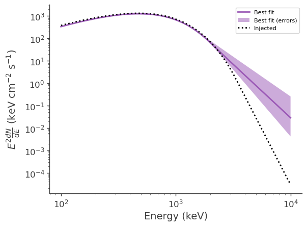
Plot the fitted and injected spectra
[16]:
fig,ax = plt.subplots()

ax.plot(energy, energy*energy*flux_median, label = "Best fit")
ax.fill_between(energy, energy*energy*flux_lo, energy*energy*flux_hi, alpha = .5, label = "Best fit (errors)")
ax.plot(energy, energy*energy*flux_inj, color = 'black', ls = ":", label = "Injected")

ax.set_xscale("log")
ax.set_yscale("log")

ax.set_xlabel("Energy (keV)")
ax.set_ylabel(r"$E^2 \frac{dN}{dE}$ (keV cm$^{-2}$ s$^{-1}$)")

ax.legend()
[16]:
<matplotlib.legend.Legend at 0x2ba21fa42d40>
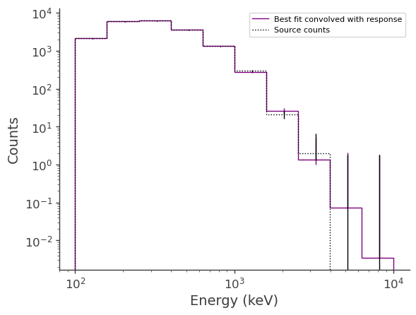
Plot the fitted spectrum convolved with the response, as well as the simulated source counts
[17]:
fit_poisson_error = np.zeros((2,len(expectation.project('Em').todense().contents)))
fit_gaussian_error = np.zeros(len(expectation.project('Em').todense().contents))
inj_poisson_error = np.zeros((2,len(grb.binned_data.project('Em').todense().contents)))
inj_gaussian_error = np.zeros(len(grb.binned_data.project('Em').todense().contents))

for i, counts in enumerate(expectation.project('Em').todense().contents):
    if counts > 5:
        fit_gaussian_error[i] = np.sqrt(counts)
    else:
        poisson_error = poisson_conf_interval(counts, interval="frequentist-confidence", sigma=1)
        fit_poisson_error[0][i] = poisson_error[0]
        fit_poisson_error[1][i] = poisson_error[1]

for i, counts in enumerate(grb.binned_data.project('Em').todense().contents):
    if counts > 5:
        inj_gaussian_error[i] = np.sqrt(counts)
    else:
        poisson_error = poisson_conf_interval(counts, interval="frequentist-confidence", sigma=1)
        inj_poisson_error[0][i] = poisson_error[0]
        inj_poisson_error[1][i] = poisson_error[1]

fig,ax = plt.subplots()

ax.stairs(expectation.project('Em').todense().contents, binned_energy_edges, color='purple', label = "Best fit convolved with response")
ax.errorbar(binned_energy, expectation.project('Em').todense().contents, yerr=fit_poisson_error, color='purple', linewidth=0, elinewidth=1)
ax.errorbar(binned_energy, expectation.project('Em').todense().contents, yerr=fit_gaussian_error, color='purple', linewidth=0, elinewidth=1)
ax.stairs(grb.binned_data.project('Em').todense().contents, binned_energy_edges, color = 'black', ls = ":", label = "Source counts")
ax.errorbar(binned_energy, grb.binned_data.project('Em').todense().contents, yerr=inj_poisson_error, color='black', linewidth=0, elinewidth=1)
ax.errorbar(binned_energy, grb.binned_data.project('Em').todense().contents, yerr=inj_gaussian_error, color='black', linewidth=0, elinewidth=1)

ax.set_xscale("log")
ax.set_yscale("log")

ax.set_xlabel("Energy (keV)")
ax.set_ylabel("Counts")

ax.legend()
[17]:
<matplotlib.legend.Legend at 0x2ba222185e40>
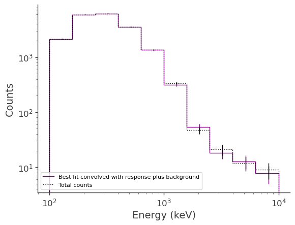
Plot the fitted spectrum convolved with the response plus the fitted background, as well as the simulated source+background counts
[18]:
fit_bkg_poisson_error = np.zeros((2,len(expectation.project('Em').todense().contents+(bkg_par.value * bkg.binned_data.slice[{'Time':slice(bkg_min,bkg_max)}].project('Em').todense().contents))))
fit_bkg_gaussian_error = np.zeros(len(expectation.project('Em').todense().contents+(bkg_par.value * bkg.binned_data.slice[{'Time':slice(bkg_min,bkg_max)}].project('Em').todense().contents)))
inj_bkg_poisson_error = np.zeros((2,len(grb_bkg.binned_data.project('Em').todense().contents)))
inj_bkg_gaussian_error = np.zeros(len(grb_bkg.binned_data.project('Em').todense().contents))

for i, counts in enumerate(expectation.project('Em').todense().contents+(bkg_par.value * bkg.binned_data.slice[{'Time':slice(bkg_min,bkg_max)}].project('Em').todense().contents)):
    if counts > 5:
        fit_bkg_gaussian_error[i] = np.sqrt(counts)
    else:
        poisson_error = poisson_conf_interval(counts, interval="frequentist-confidence", sigma=1)
        fit_bkg_poisson_error[0][i] = poisson_error[0]
        fit_bkg_poisson_error[1][i] = poisson_error[1]

for i, counts in enumerate(grb_bkg.binned_data.project('Em').todense().contents):
    if counts > 5:
        inj_bkg_gaussian_error[i] = np.sqrt(counts)
    else:
        poisson_error = poisson_conf_interval(counts, interval="frequentist-confidence", sigma=1)
        inj_bkg_poisson_error[0][i] = poisson_error[0]
        inj_bkg_poisson_error[1][i] = poisson_error[1]

fig,ax = plt.subplots()

ax.stairs(expectation.project('Em').todense().contents+(bkg_par.value * bkg.binned_data.slice[{'Time':slice(bkg_min,bkg_max)}].project('Em').todense().contents), binned_energy_edges, color='purple', label = "Best fit convolved with response plus background")
ax.errorbar(binned_energy, expectation.project('Em').todense().contents+(bkg_par.value * bkg.binned_data.slice[{'Time':slice(bkg_min,bkg_max)}].project('Em').todense().contents), yerr=fit_bkg_poisson_error, color='purple', linewidth=0, elinewidth=1)
ax.errorbar(binned_energy, expectation.project('Em').todense().contents+(bkg_par.value * bkg.binned_data.slice[{'Time':slice(bkg_min,bkg_max)}].project('Em').todense().contents), yerr=fit_bkg_gaussian_error, color='purple', linewidth=0, elinewidth=1)
ax.stairs(grb_bkg.binned_data.project('Em').todense().contents, binned_energy_edges, color = 'black', ls = ":", label = "Total counts")
ax.errorbar(binned_energy, grb_bkg.binned_data.project('Em').todense().contents, yerr=inj_bkg_poisson_error, color='black', linewidth=0, elinewidth=1)
ax.errorbar(binned_energy, grb_bkg.binned_data.project('Em').todense().contents, yerr=inj_bkg_gaussian_error, color='black', linewidth=0, elinewidth=1)

ax.set_xscale("log")
ax.set_yscale("log")

ax.set_xlabel("Energy (keV)")
ax.set_ylabel("Counts")

ax.legend()
[18]:
<matplotlib.legend.Legend at 0x2ba221d57460>