Line Background Estimation Using Adjacent Energy Bins

H.Yoneda, S. Mittal

This is a tutorial notebook on background estimation for gamma-ray lines. The basic idea is as follows:

Extracting the event distribution in the Compton data space from adjacent energy bins of the energy of interest.
Making a binned histogram using the extracted events.
Estimate the total number of expected background counts in the line energy bin by fitting the adjacent energy bin data, and modify the normalization of the binned histogram accordingly.

Here, we make a background model for Al-26. These processes will be performed in the LineBackgroundEstimation class, and you can see how it works as follows.

This class is very preliminary, and there are several areas for improvement. Future ideas include:

We may add more options in the minuit fitting, e.g., limiting the parameter region, fixing some parameters.
We may apply smoothing to the background histogram, which may help to mitigate Poisson fluctuation in the model.

[1]:

import logging
import sys
logger = logging.getLogger('cosipy')
logger.setLevel(logging.INFO)
logger.addHandler(logging.StreamHandler(sys.stdout))

[3]:

from histpy import Histogram, Axis, Axes
import astropy.units as u
import numpy as np
import matplotlib.pyplot as plt
from scipy.optimize import curve_fit
from scipy import integrate
from iminuit import Minuit
from cosipy import BinnedData, LineBackgroundEstimation

[4]:

%matplotlib inline
%config InlineBackend.figure_format='retina'

0. Create dataset for the line background estimation

We need an event histogram binned finely along the energy axis.

[5]:

#need to change them
path_to_Al  = "path/to/data"
path_to_bkg = "path/to/data"

[5]:

#yaml files containing binning information
spectrum_bkg = BinnedData("inputs_bkg_estimation.yaml")
spectrum_Al = BinnedData("inputs_bkg_estimation.yaml")

[6]:

%%time

#path to unbinned fits file for source and background to create binned dataset
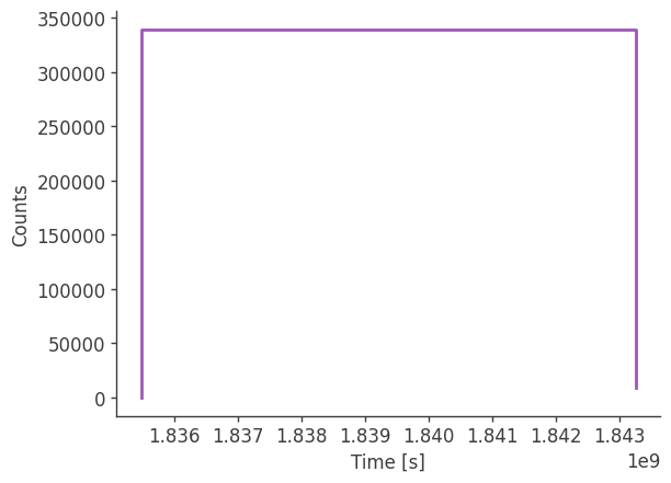
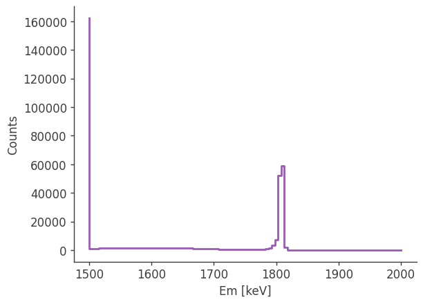
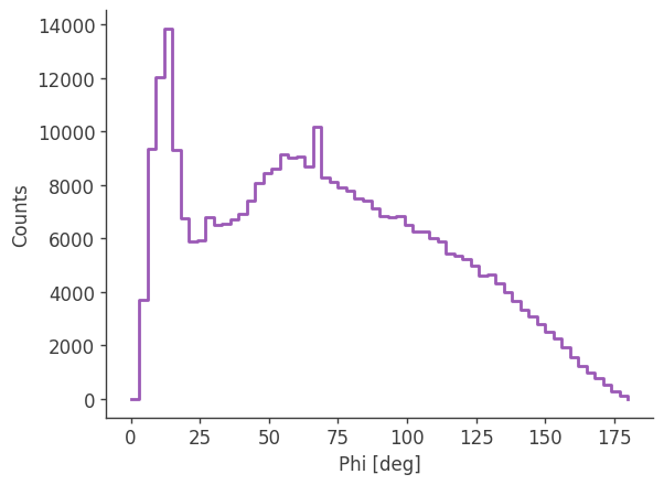
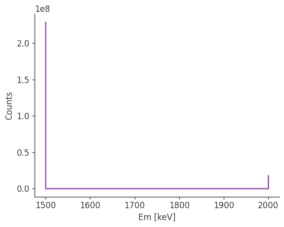
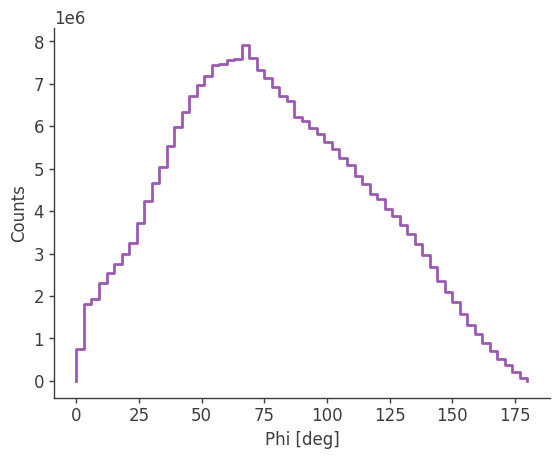
spectrum_Al.get_binned_data(unbinned_data=path_to_Al, make_binning_plots=True,
            output_name='Al_binned', show_plots=True)

binning data...
Time unit: s
Em unit: keV
Phi unit: deg
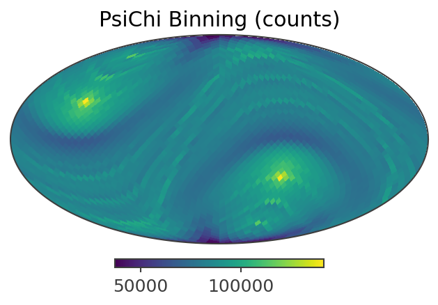
PsiChi unit: None

../../../_images/tutorials_background_estimation_line_background_line_background_estimation_example_notebook_7_1.png

../../../_images/tutorials_background_estimation_line_background_line_background_estimation_example_notebook_7_2.png

../../../_images/tutorials_background_estimation_line_background_line_background_estimation_example_notebook_7_3.png

../../../_images/tutorials_background_estimation_line_background_line_background_estimation_example_notebook_7_4.png

../../../_images/tutorials_background_estimation_line_background_line_background_estimation_example_notebook_7_5.png

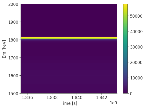
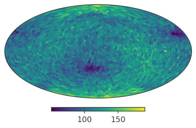
plotting psichi in Galactic coordinates...

../../../_images/tutorials_background_estimation_line_background_line_background_estimation_example_notebook_7_7.png

CPU times: user 6.48 s, sys: 1.73 s, total: 8.21 s
Wall time: 4.5 s

[7]:

%%time

#path to unbinned fits file for source and background to create binned dataset
spectrum_bkg.get_binned_data(unbinned_data=path_to_bkg, make_binning_plots=True,
            output_name='bkg_binned', show_plots=True)

binning data...
Time unit: s
Em unit: keV
Phi unit: deg
PsiChi unit: None

../../../_images/tutorials_background_estimation_line_background_line_background_estimation_example_notebook_8_1.png

../../../_images/tutorials_background_estimation_line_background_line_background_estimation_example_notebook_8_2.png

../../../_images/tutorials_background_estimation_line_background_line_background_estimation_example_notebook_8_3.png

../../../_images/tutorials_background_estimation_line_background_line_background_estimation_example_notebook_8_4.png

../../../_images/tutorials_background_estimation_line_background_line_background_estimation_example_notebook_8_5.png

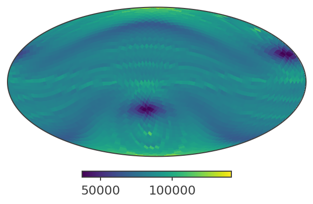
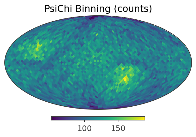
plotting psichi in Galactic coordinates...

../../../_images/tutorials_background_estimation_line_background_line_background_estimation_example_notebook_8_7.png

CPU times: user 10min 9s, sys: 46.7 s, total: 10min 56s
Wall time: 11min 53s

[8]:

#combine source and background binned data
spectrum_total = spectrum_Al.binned_data + spectrum_bkg.binned_data
spectrum_total.write('combined_al_bkg_nside_16.hdf5')

This spectrum_total can be considered as the actual event histogram in COSI observations.

[7]:

# load data
spectrum_bkg = Histogram.open("bkg_binned.hdf5")
spectrum_Al = Histogram.open("Al_binned.hdf5")
spectrum_total = Histogram.open("combined_al_bkg_nside_16.hdf5")

1. Instantiate the LineBackgroundEstimation

[8]:

instance = LineBackgroundEstimation(spectrum_total)

2. Set background model and fit it

Define a background spectrum model for fitting data

[9]:

def powerlaw(x, a, b, pivot):
    return a * (x/pivot)**b

def gaussian(x, a, mu, sigma):
    return a / (sigma) / np.sqrt(2 * np.pi) * np.exp( -(x-mu)**2 / (2*sigma**2))

def bkg_model(x, a, b, a1, mu1, a2, mu2, a3, mu3, a4, mu4, sigma):
    pivot = 1800.0
    return powerlaw(x,a,b, pivot) + \
            gaussian(x , a1, mu1, sigma) + \
            gaussian(x , a2, mu2, sigma) + \
            gaussian(x , a3, mu3, sigma) + \
            gaussian(x , a4, mu4, sigma)

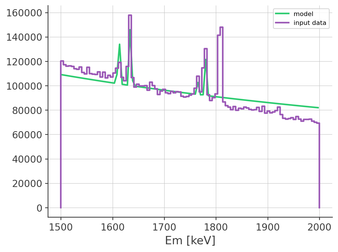
[10]:

instance.set_bkg_energy_spectrum_model(bkg_model, [18000.0, -1.0, 40000.0, 1612, 50000.0, 1635, 10000.0, 1765, 30000.0, 1780, 1.0])
instance.plot_energy_spectrum()

[10]:

(<Axes: xlabel='Em [keV]'>, <ErrorbarContainer object of 3 artists>)

../../../_images/tutorials_background_estimation_line_background_line_background_estimation_example_notebook_17_1.png

[11]:

%%time

m = instance.fit_energy_spectrum()
m

CPU times: user 12.9 s, sys: 92.6 ms, total: 13 s
Wall time: 13.1 s

[11]:

Migrad
FCN = -9.903e+07	Nfcn = 1293
EDM = 0.000122 (Goal: 0.0001)
Valid Minimum	Below EDM threshold (goal x 10)
No parameters at limit	Below call limit
Hesse ok	Covariance accurate

	Name	Value	Hesse Error	Minos Error-	Minos Error+	Limit-	Limit+	Fixed
0	x0	17.385e3	0.007e3
1	x1	-1.702	0.004
2	x2	21.7e3	0.5e3
3	x3	1.61183e3	0.00007e3
4	x4	71.7e3	0.6e3
5	x5	1.633314e3	0.000034e3
6	x6	24.8e3	0.5e3
7	x7	1.76410e3	0.00009e3
8	x8	67.2e3	0.5e3
9	x9	1.778490e3	0.000025e3
10	x10	2.136	0.027

	x0	x1	x2	x3	x4	x5	x6	x7	x8	x9	x10
x0	45.1	11.407e-3 (0.422)	-340 (-0.101)	-0.004 (-0.009)	-640 (-0.152)	-0.0103 (-0.046)	-520 (-0.165)	-0.009 (-0.015)	-600 (-0.169)	-8.5e-3 (-0.050)	-28.8e-3 (-0.158)
x1	11.407e-3 (0.422)	1.62e-05	260.031e-3 (0.128)	-0.005e-3 (-0.018)	256.797e-3 (0.102)	0 (0.003)	-36.617e-3 (-0.019)	0.009e-3 (0.026)	-52.712e-3 (-0.025)	0.003e-3 (0.031)	0.007e-3 (0.060)
x2	-340 (-0.101)	260.031e-3 (0.128)	2.54e+05	-5.590 (-0.156)	0.03e6 (0.098)	0.7165 (0.042)	0.01e6 (0.044)	1.714 (0.039)	0.01e6 (0.049)	713.3e-3 (0.056)	1.8033 (0.132)
x3	-0.004 (-0.009)	-0.005e-3 (-0.018)	-5.590 (-0.156)	0.00508	3.384 (0.076)	0.0001 (0.054)	0.915 (0.027)	0.000 (0.049)	1.405 (0.037)	0.1e-3 (0.064)	0.3e-3 (0.144)
x4	-640 (-0.152)	256.797e-3 (0.102)	0.03e6 (0.098)	3.384 (0.076)	3.91e+05	1.9929 (0.095)	0.04e6 (0.130)	10.077 (0.184)	0.05e6 (0.164)	3.9090 (0.246)	9.5317 (0.561)
x5	-0.0103 (-0.046)	0 (0.003)	0.7165 (0.042)	0.0001 (0.054)	1.9929 (0.095)	0.00113	1.1696 (0.074)	0.0004 (0.123)	1.7470 (0.098)	0.1e-3 (0.161)	0.3e-3 (0.364)
x6	-520 (-0.165)	-36.617e-3 (-0.019)	0.01e6 (0.044)	0.915 (0.027)	0.04e6 (0.130)	1.1696 (0.074)	2.2e+05	-7.432 (-0.182)	0.02e6 (0.075)	1.0703 (0.090)	2.6815 (0.211)
x7	-0.009 (-0.015)	0.009e-3 (0.026)	1.714 (0.039)	0.000 (0.049)	10.077 (0.184)	0.0004 (0.123)	-7.432 (-0.182)	0.00763	3.914 (0.085)	0.3e-3 (0.156)	0.8e-3 (0.336)
x8	-600 (-0.169)	-52.712e-3 (-0.025)	0.01e6 (0.049)	1.405 (0.037)	0.05e6 (0.164)	1.7470 (0.098)	0.02e6 (0.075)	3.914 (0.085)	2.79e+05	117.0e-3 (0.009)	3.9541 (0.276)
x9	-8.5e-3 (-0.050)	0.003e-3 (0.031)	713.3e-3 (0.056)	0.1e-3 (0.064)	3.9090 (0.246)	0.1e-3 (0.161)	1.0703 (0.090)	0.3e-3 (0.156)	117.0e-3 (0.009)	0.000647	0.3e-3 (0.441)
x10	-28.8e-3 (-0.158)	0.007e-3 (0.060)	1.8033 (0.132)	0.3e-3 (0.144)	9.5317 (0.561)	0.3e-3 (0.364)	2.6815 (0.211)	0.8e-3 (0.336)	3.9541 (0.276)	0.3e-3 (0.441)	0.000739

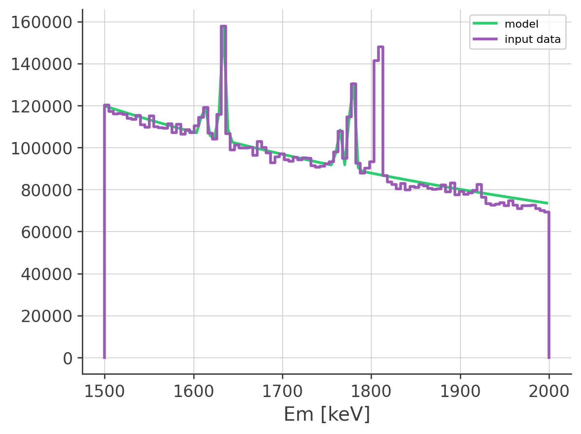
[12]:

ax, _ = instance.plot_energy_spectrum()

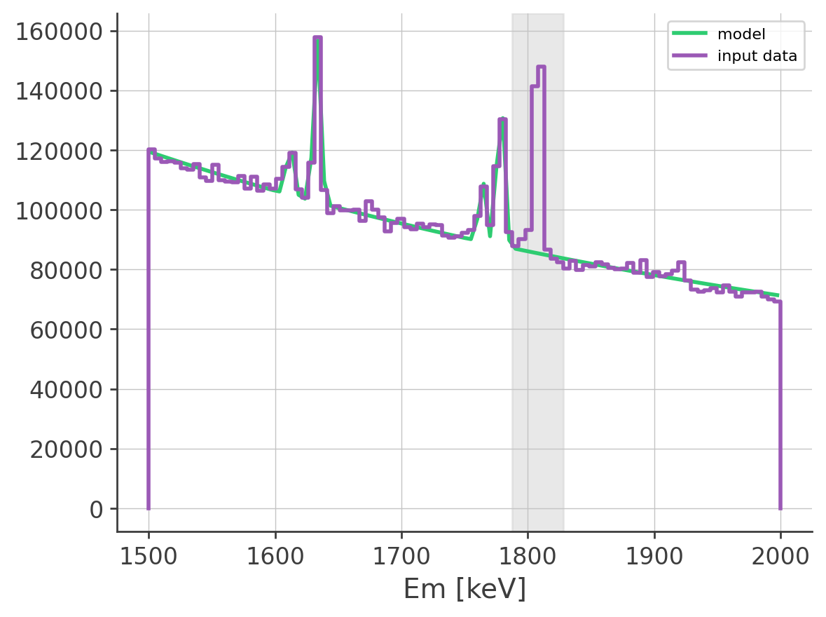
../../../_images/tutorials_background_estimation_line_background_line_background_estimation_example_notebook_19_0.png

Mask a region around Al-26

[13]:

instance.set_mask((1790.0, 1825.0) * u.keV)
instance.mask

[13]:

array([False, False, False, False, False, False, False, False, False,
       False, False, False, False, False, False, False, False, False,
       False, False, False, False, False, False, False, False, False,
       False, False, False, False, False, False, False, False, False,
       False, False, False, False, False, False, False, False, False,
       False, False, False, False, False, False, False, False, False,
       False, False, False,  True,  True,  True,  True,  True,  True,
        True,  True, False, False, False, False, False, False, False,
       False, False, False, False, False, False, False, False, False,
       False, False, False, False, False, False, False, False, False,
       False, False, False, False, False, False, False, False, False])

[14]:

m = instance.fit_energy_spectrum()
m

[14]:

Migrad
FCN = -9.049e+07	Nfcn = 933
EDM = 0.00035 (Goal: 0.0001)
Valid Minimum	Below EDM threshold (goal x 10)
No parameters at limit	Below call limit
Hesse ok	Covariance accurate

	Name	Value	Hesse Error	Minos Error-	Minos Error+	Limit-	Limit+	Fixed
0	x0	17.041e3	0.007e3
1	x1	-1.797	0.004
2	x2	24.3e3	0.5e3
3	x3	1.61187e3	0.00007e3
4	x4	76.4e3	0.6e3
5	x5	1.633376e3	0.000030e3
6	x6	28.9e3	0.5e3
7	x7	1.76417e3	0.00008e3
8	x8	72.0e3	0.5e3
9	x9	1.778556e3	0.000027e3
10	x10	2.347	0.024

	x0	x1	x2	x3	x4	x5	x6	x7	x8	x9	x10
x0	50.2	13.120e-3 (0.450)	-410 (-0.114)	-0.006 (-0.011)	-710 (-0.163)	-6.9e-3 (-0.032)	-630 (-0.185)	-0.012 (-0.021)	-740 (-0.191)	-10.4e-3 (-0.055)	-31.4e-3 (-0.182)
x1	13.120e-3 (0.450)	1.69e-05	255.291e-3 (0.121)	-0.005e-3 (-0.018)	223.419e-3 (0.088)	-0.001e-3 (-0.005)	-59.125e-3 (-0.030)	0.005e-3 (0.016)	-79.896e-3 (-0.036)	0.002e-3 (0.018)	0.004e-3 (0.038)
x2	-410 (-0.114)	255.291e-3 (0.121)	2.64e+05	-4.513 (-0.119)	0.03e6 (0.109)	486.9e-3 (0.032)	0.01e6 (0.060)	1.787 (0.042)	0.02e6 (0.068)	837.5e-3 (0.061)	2.0392 (0.163)
x3	-0.006 (-0.011)	-0.005e-3 (-0.018)	-4.513 (-0.119)	0.00544	2.659 (0.058)	0.1e-3 (0.028)	1.056 (0.030)	0.000 (0.036)	1.563 (0.039)	0.1e-3 (0.049)	0.2e-3 (0.124)
x4	-710 (-0.163)	223.419e-3 (0.088)	0.03e6 (0.109)	2.659 (0.058)	3.83e+05	727.7e-3 (0.039)	0.04e6 (0.145)	7.219 (0.139)	0.06e6 (0.178)	3.2111 (0.196)	7.6133 (0.505)
x5	-6.9e-3 (-0.032)	-0.001e-3 (-0.005)	486.9e-3 (0.032)	0.1e-3 (0.028)	727.7e-3 (0.039)	0.000905	799.9e-3 (0.055)	0.2e-3 (0.062)	1.1569 (0.070)	0.1e-3 (0.085)	0.2e-3 (0.218)
x6	-630 (-0.185)	-59.125e-3 (-0.030)	0.01e6 (0.060)	1.056 (0.030)	0.04e6 (0.145)	799.9e-3 (0.055)	2.33e+05	-4.481 (-0.111)	0.03e6 (0.105)	1.2824 (0.100)	3.0630 (0.261)
x7	-0.012 (-0.021)	0.005e-3 (0.016)	1.787 (0.042)	0.000 (0.036)	7.219 (0.139)	0.2e-3 (0.062)	-4.481 (-0.111)	0.007	3.761 (0.082)	0.3e-3 (0.129)	0.6e-3 (0.283)
x8	-740 (-0.191)	-79.896e-3 (-0.036)	0.02e6 (0.068)	1.563 (0.039)	0.06e6 (0.178)	1.1569 (0.070)	0.03e6 (0.105)	3.761 (0.082)	2.98e+05	626.6e-3 (0.043)	4.3838 (0.330)
x9	-10.4e-3 (-0.055)	0.002e-3 (0.018)	837.5e-3 (0.061)	0.1e-3 (0.049)	3.2111 (0.196)	0.1e-3 (0.085)	1.2824 (0.100)	0.3e-3 (0.129)	626.6e-3 (0.043)	0.000704	0.3e-3 (0.390)
x10	-31.4e-3 (-0.182)	0.004e-3 (0.038)	2.0392 (0.163)	0.2e-3 (0.124)	7.6133 (0.505)	0.2e-3 (0.218)	3.0630 (0.261)	0.6e-3 (0.283)	4.3838 (0.330)	0.3e-3 (0.390)	0.000594

[15]:

ax, _ = instance.plot_energy_spectrum()

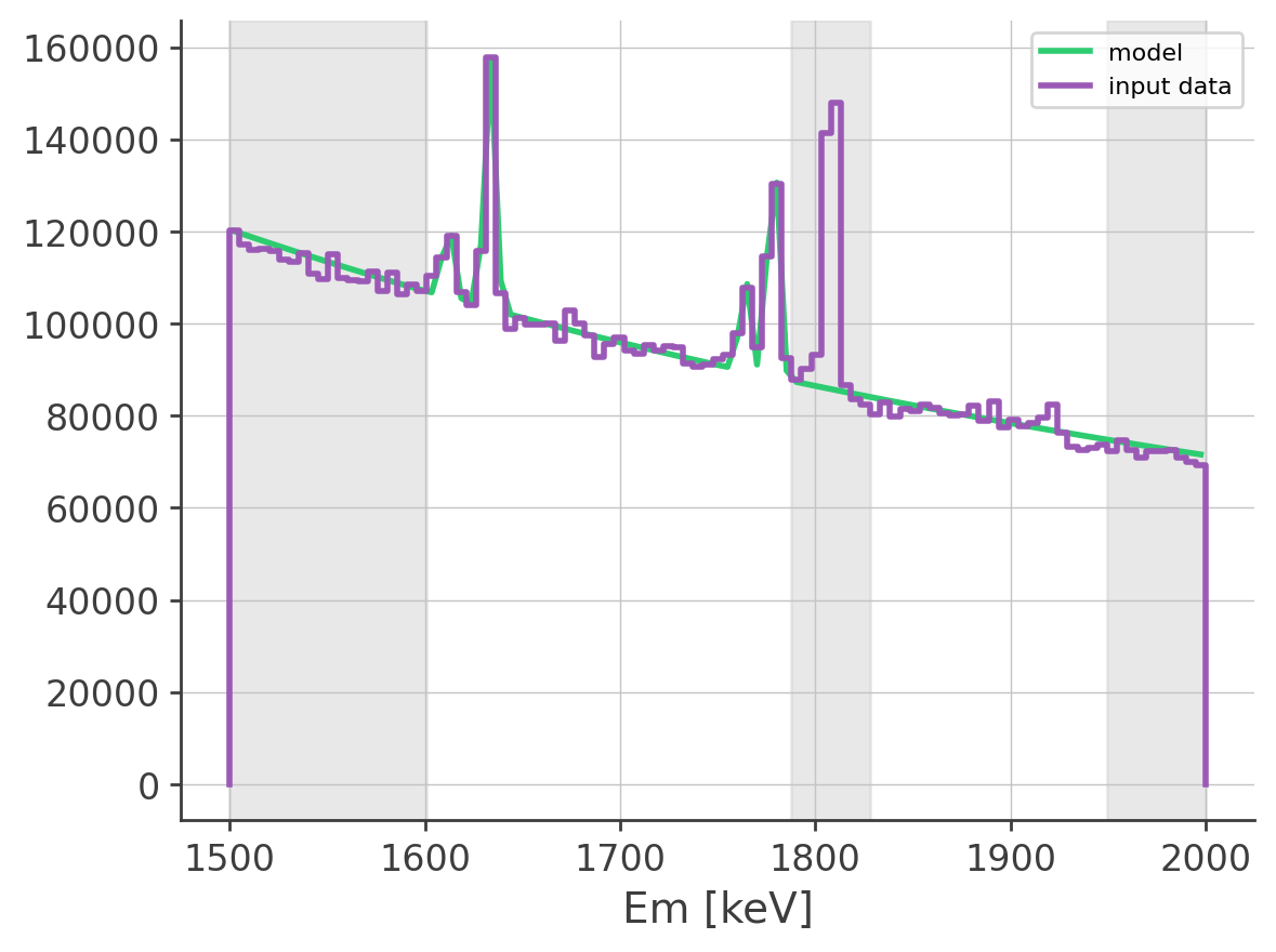
../../../_images/tutorials_background_estimation_line_background_line_background_estimation_example_notebook_23_0.png

Mask more

[16]:

instance.set_mask((1790.0, 1825.0) * u.keV, (1500.0, 1600.0) * u.keV, (1950.0, 2000.0) * u.keV)
instance.mask

[16]:

array([ True,  True,  True,  True,  True,  True,  True,  True,  True,
        True,  True,  True,  True,  True,  True,  True,  True,  True,
        True,  True, False, False, False, False, False, False, False,
       False, False, False, False, False, False, False, False, False,
       False, False, False, False, False, False, False, False, False,
       False, False, False, False, False, False, False, False, False,
       False, False, False,  True,  True,  True,  True,  True,  True,
        True,  True, False, False, False, False, False, False, False,
       False, False, False, False, False, False, False, False, False,
       False, False, False, False, False, False, False, False,  True,
        True,  True,  True,  True,  True,  True,  True,  True,  True])

[17]:

m = instance.fit_energy_spectrum()
m

[17]:

Migrad
FCN = -5.934e+07	Nfcn = 932
EDM = 0.000404 (Goal: 0.0001)
Valid Minimum	Below EDM threshold (goal x 10)
No parameters at limit	Below call limit
Hesse ok	Covariance accurate

	Name	Value	Hesse Error	Minos Error-	Minos Error+	Limit-	Limit+	Fixed
0	x0	17.119e3	0.008e3
1	x1	-1.816	0.008
2	x2	22.6e3	0.5e3
3	x3	1.61187e3	0.00007e3
4	x4	74.1e3	0.7e3
5	x5	1.633360e3	0.000031e3
6	x6	27.6e3	0.5e3
7	x7	1.76412e3	0.00008e3
8	x8	70.5e3	0.5e3
9	x9	1.778526e3	0.000026e3
10	x10	2.262	0.027

	x0	x1	x2	x3	x4	x5	x6	x7	x8	x9	x10
x0	71.6	15.55e-3 (0.230)	-650 (-0.141)	-0.007 (-0.011)	-1.12e3 (-0.200)	-12.5e-3 (-0.047)	-900 (-0.220)	-0.022 (-0.031)	-1.05e3 (-0.226)	-16.1e-3 (-0.073)	-49.1e-3 (-0.217)
x1	15.55e-3 (0.230)	6.39e-05	1.46470 (0.337)	-0.02e-3 (-0.035)	1.62313 (0.306)	0 (0.020)	267.55e-3 (0.069)	0.04e-3 (0.062)	266.40e-3 (0.061)	0.02e-3 (0.092)	0.05e-3 (0.221)
x2	-650 (-0.141)	1.46470 (0.337)	2.95e+05	-5.593 (-0.138)	0.08e6 (0.212)	761e-3 (0.045)	0.03e6 (0.098)	2.909 (0.063)	0.03e6 (0.104)	1.3286 (0.093)	3.3261 (0.229)
x3	-0.007 (-0.011)	-0.02e-3 (-0.035)	-5.593 (-0.138)	0.00557	2.547 (0.052)	0.1e-3 (0.035)	0.944 (0.026)	0.000 (0.041)	1.468 (0.036)	0.1e-3 (0.052)	0.2e-3 (0.118)
x4	-1.12e3 (-0.200)	1.62313 (0.306)	0.08e6 (0.212)	2.547 (0.052)	4.39e+05	1.3646 (0.066)	0.06e6 (0.184)	10.071 (0.180)	0.08e6 (0.216)	4.2213 (0.243)	10.1576 (0.574)
x5	-12.5e-3 (-0.047)	0 (0.020)	761e-3 (0.045)	0.1e-3 (0.035)	1.3646 (0.066)	0.000979	1.0465 (0.069)	0.2e-3 (0.088)	1.5065 (0.088)	0.1e-3 (0.115)	0.2e-3 (0.265)
x6	-900 (-0.220)	267.55e-3 (0.069)	0.03e6 (0.098)	0.944 (0.026)	0.06e6 (0.184)	1.0465 (0.069)	2.35e+05	-4.936 (-0.120)	0.03e6 (0.122)	1.4595 (0.115)	3.5779 (0.277)
x7	-0.022 (-0.031)	0.04e-3 (0.062)	2.909 (0.063)	0.000 (0.041)	10.071 (0.180)	0.2e-3 (0.088)	-4.936 (-0.120)	0.00716	4.655 (0.100)	0.3e-3 (0.154)	0.7e-3 (0.327)
x8	-1.05e3 (-0.226)	266.40e-3 (0.061)	0.03e6 (0.104)	1.468 (0.036)	0.08e6 (0.216)	1.5065 (0.088)	0.03e6 (0.122)	4.655 (0.100)	3e+05	757.8e-3 (0.053)	5.0118 (0.343)
x9	-16.1e-3 (-0.073)	0.02e-3 (0.092)	1.3286 (0.093)	0.1e-3 (0.052)	4.2213 (0.243)	0.1e-3 (0.115)	1.4595 (0.115)	0.3e-3 (0.154)	757.8e-3 (0.053)	0.000686	0.3e-3 (0.430)
x10	-49.1e-3 (-0.217)	0.05e-3 (0.221)	3.3261 (0.229)	0.2e-3 (0.118)	10.1576 (0.574)	0.2e-3 (0.265)	3.5779 (0.277)	0.7e-3 (0.327)	5.0118 (0.343)	0.3e-3 (0.430)	0.000713

[18]:

ax, _ = instance.plot_energy_spectrum()

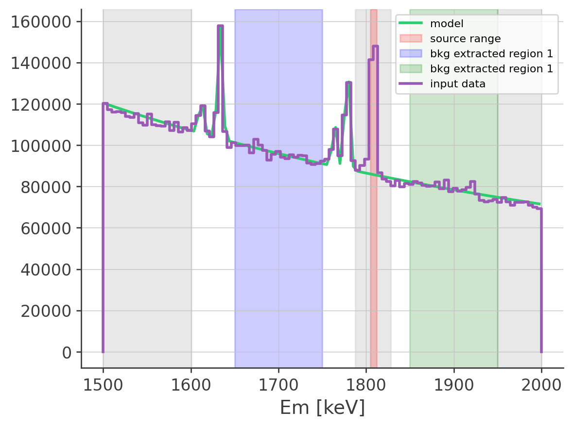
../../../_images/tutorials_background_estimation_line_background_line_background_estimation_example_notebook_27_0.png

3. Generate Background Histogram

[38]:

source_range = (1805, 1812)  * u.keV #counts estimation in Al26 line

background_region_1 = (1650, 1750) * u.keV #background counts estimation before the line
background_region_2 = (1850, 1950) * u.keV #background counts estimation before the line

[39]:

bkg_model_histogram = instance.generate_bkg_model_histogram(source_range, [background_region_1, background_region_2])

The energy range [1650. 1750.] is modified to [1651.51515152, 1747.47474747]
The energy range [1850. 1950.] is modified to [1853.53535354, 1949.49494949]

[40]:

ax, _ = instance.plot_energy_spectrum()

ax.axvspan(source_range[0].value, source_range[1].value, color='red', alpha=0.2, label = 'source range')

ax.axvspan(background_region_1[0].value, background_region_1[1].value, color='blue', alpha=0.2, label = 'bkg extracted region 1')
ax.axvspan(background_region_2[0].value, background_region_2[1].value, color='green', alpha=0.2, label = 'bkg extracted region 1')

ax.legend()

[40]:

<matplotlib.legend.Legend at 0x3c1cbee90>

../../../_images/tutorials_background_estimation_line_background_line_background_estimation_example_notebook_31_1.png

[41]:

bkg_model_histogram.write('bkg_model_al26_line.hdf5', overwrite=True)

4. Compare the background model with the actual background data

[24]:

%%time

bkg_histogram_in_Al26line = BinnedData("inputs_check_results.yaml")
bkg_histogram_in_Al26line.get_binned_data(unbinned_data=path_to_bkg, make_binning_plots=False,
                                          output_name='bkg_data_al26_line_for_comparison', show_plots=False)

binning data...
Time unit: s
Em unit: keV
Phi unit: deg
PsiChi unit: None
CPU times: user 9min 42s, sys: 43.6 s, total: 10min 26s
Wall time: 11min 21s

[42]:

bkg_histogram_in_Al26line = Histogram.open("bkg_data_al26_line_for_comparison.hdf5")

[43]:

bkg_model_histogram = bkg_model_histogram.todense()
bkg_histogram_in_Al26line = bkg_histogram_in_Al26line.todense()

[44]:

bkg_model_histogram.clear_underflow_and_overflow()
bkg_histogram_in_Al26line.clear_underflow_and_overflow()

Normalization

[45]:

count_model = np.sum(bkg_model_histogram[:])
count_obs = np.sum(bkg_histogram_in_Al26line[:])

print("model:", count_model)
print("data:", count_obs)
print("difference:", (count_obs/count_model - 1)*1e2, "%")

model: 115660.74857012795
data: 121530.0
difference: 5.074540414472062 %

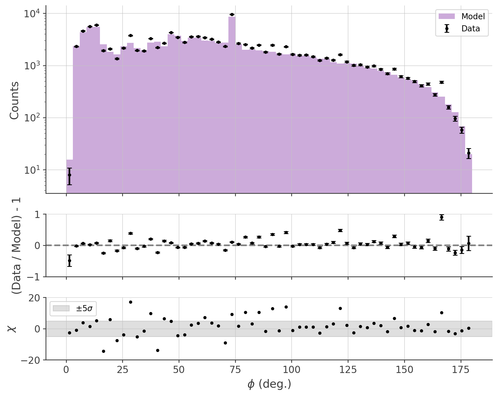
Phi distritbuion

[46]:

bkg_model_phi = bkg_model_histogram.project("Phi").todense()
bkg_obs_phi = bkg_histogram_in_Al26line.project("Phi").todense()

[47]:

fig, (ax1, ax2, ax3) = plt.subplots(3, 1, figsize=(10, 8), sharex=True, gridspec_kw={'height_ratios': [3, 1, 1]})

ax3.set_xlabel(r'$\phi$ (deg.)')

ax1.bar(bkg_model_phi.axis.centers, bkg_model_phi.contents, width = 3, alpha=0.5, label='Model')
#ax1.bar(bkg_obs_phi.axis.centers,   bkg_obs_phi.contents,   width = 3, alpha=0.5, label='Data', capsize=3, yerr = np.sqrt(bkg_obs_phi.contents))
ax1.errorbar(bkg_obs_phi.axis.centers, bkg_obs_phi.contents, color = 'black', label='Data', fmt='.', capsize=3, yerr = np.sqrt(bkg_obs_phi.contents))
ax1.set_ylabel('Counts')
ax1.legend(fontsize = 10)
ax1.grid()
ax1.set_yscale('log')

# ratio
diff = bkg_obs_phi.contents / bkg_model_phi.contents - 1
diff_err = np.sqrt(bkg_obs_phi.contents) / bkg_model_phi.contents
ax2.errorbar(bkg_model_phi.axis.centers, diff, yerr=diff_err, fmt='.', capsize=3, color = 'black')
ax2.axhline(y = 0, color = 'grey', linestyle = '--')
ax2.grid()
ax2.set_ylabel('(Data / Model) - 1')
ax2.set_ylim(-1, 1)

# chi
xi = (bkg_obs_phi.contents - bkg_model_phi.contents) / np.sqrt(bkg_obs_phi.contents)
ax3.plot(bkg_model_phi.axis.centers, xi, '.', color = 'black')
ax3.axhspan(-5, 5, color = 'grey', alpha = 0.25, label = r"$\pm 5 \sigma$")
ax3.set_ylabel(r"$\chi$")
ax3.grid()
ax3.legend(fontsize = 10)
ax3.set_ylim(-20, 20)

[47]:

(-20.0, 20.0)

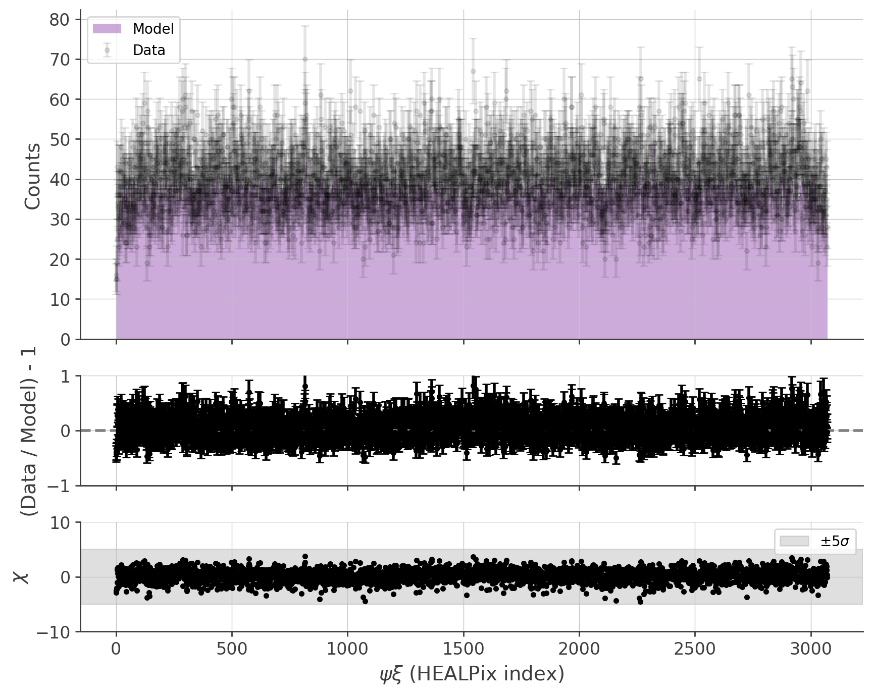
../../../_images/tutorials_background_estimation_line_background_line_background_estimation_example_notebook_42_1.png

PsiChi distritbuion

[48]:

bkg_model_psichi = bkg_model_histogram.project("PsiChi")
bkg_obs_psichi = bkg_histogram_in_Al26line.project("PsiChi")

[49]:

fig, (ax1, ax2, ax3) = plt.subplots(3, 1, figsize=(10, 8), sharex=True, gridspec_kw={'height_ratios': [3, 1, 1]})

ax3.set_xlabel(r'$\psi \xi$ (HEALPix index)')

ax1.bar(bkg_model_psichi.axis.centers, bkg_model_psichi.contents, width = 1, alpha=0.5, label='Model')
#ax1.bar(bkg_obs_psichi.axis.centers,   bkg_obs_psichi.contents,   width = 3, alpha=0.5, label='Data')#, capsize=3, yerr = np.sqrt(bkg_obs_psichi.contents))
ax1.errorbar(bkg_obs_psichi.axis.centers, bkg_obs_psichi.contents, color = 'black', alpha=0.1, label='Data', fmt='.', capsize=3, yerr = np.sqrt(bkg_obs_psichi.contents))
ax1.set_ylabel('Counts')
ax1.legend(fontsize = 10)
ax1.grid()
#ax1.set_yscale('log')

# ratio
diff = bkg_obs_psichi.contents / bkg_model_psichi.contents - 1
diff_err = np.sqrt(bkg_obs_psichi.contents) / bkg_model_psichi.contents
ax2.errorbar(bkg_model_psichi.axis.centers, diff, yerr=diff_err, fmt='.', capsize=3, color = 'black')
ax2.axhline(y = 0, color = 'grey', linestyle = '--')
ax2.grid()
ax2.set_ylabel('(Data / Model) - 1')
ax2.set_ylim(-1, 1)

# chi
xi = (bkg_obs_psichi.contents - bkg_model_psichi.contents) / np.sqrt(bkg_obs_psichi.contents)
ax3.plot(bkg_model_psichi.axis.centers, xi, '.', color = 'black')
ax3.axhspan(-5, 5, color = 'grey', alpha = 0.25, label = r"$\pm 5 \sigma$")
ax3.set_ylabel(r"$\chi$")
ax3.grid()
ax3.legend(fontsize = 10)
ax3.set_ylim(-10, 10)

[49]:

(-10.0, 10.0)

../../../_images/tutorials_background_estimation_line_background_line_background_estimation_example_notebook_45_1.png

Rebinning

[50]:

import healpy as hp

[51]:

nside_out = 4

bkg_model_psichi_rebinned = hp.ud_grade(bkg_model_psichi[:], nside_out, power = -2)
bkg_obs_psichi_rebinned   = hp.ud_grade(bkg_obs_psichi[:],   nside_out, power = -2)

[52]:

fig, (ax1, ax2, ax3) = plt.subplots(3, 1, figsize=(10, 8), sharex=True, gridspec_kw={'height_ratios': [3, 1, 1]})

ax3.set_xlabel(r'$\psi \xi$ (HEALPix index)')

ax1.bar(np.arange(hp.nside2npix(nside_out)), bkg_model_psichi_rebinned, width = 1, alpha=0.5, label='Model')
#ax1.bar(np.arange(hp.nside2npix(nside_out)), bkg_obs_psichi_rebinned,   width = 3, alpha=0.5, label='Data', capsize=3, yerr = np.sqrt(bkg_obs_psichi_rebinned))
ax1.errorbar(np.arange(hp.nside2npix(nside_out)), bkg_obs_psichi_rebinned, color = 'black', alpha=1, label='Data', fmt='.', capsize=3, yerr = np.sqrt(bkg_obs_psichi_rebinned))
ax1.set_ylabel('Counts')
ax1.legend(fontsize = 10)
ax1.grid()
#ax1.set_yscale('log')

# ratio
diff = bkg_obs_psichi_rebinned / bkg_model_psichi_rebinned - 1
diff_err = np.sqrt(bkg_model_psichi_rebinned) / bkg_obs_psichi_rebinned
ax2.errorbar(np.arange(hp.nside2npix(nside_out)), diff, yerr=diff_err, fmt='.', capsize=3, color = 'black')
ax2.axhline(y = 0, color = 'grey', linestyle = '--')
ax2.grid()
ax2.set_ylabel('(Data / Model) - 1')
ax2.set_ylim(-0.3, 0.3)

# chi
xi = (bkg_obs_psichi_rebinned - bkg_model_psichi_rebinned) / np.sqrt(bkg_obs_psichi_rebinned)
ax3.plot(np.arange(hp.nside2npix(nside_out)), xi, '.', color = 'black')
ax3.axhspan(-5, 5, color = 'grey', alpha = 0.25, label = r"$\pm 5 \sigma$")
ax3.set_ylabel(r"$\chi$")
ax3.grid()
ax3.legend(fontsize = 10)
ax3.set_ylim(-10, 10)

[52]:

(-10.0, 10.0)

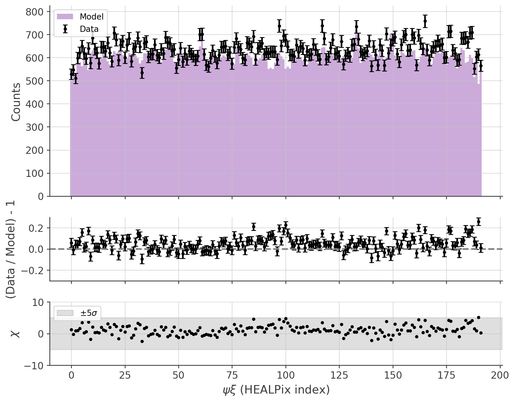
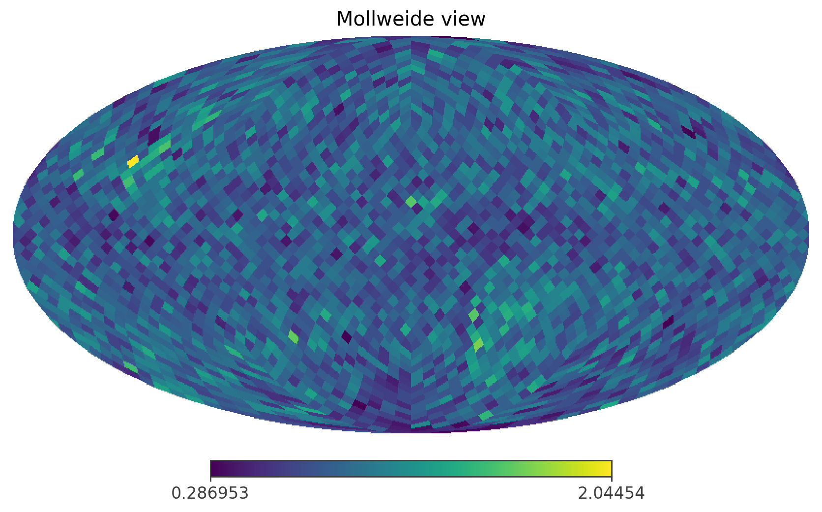
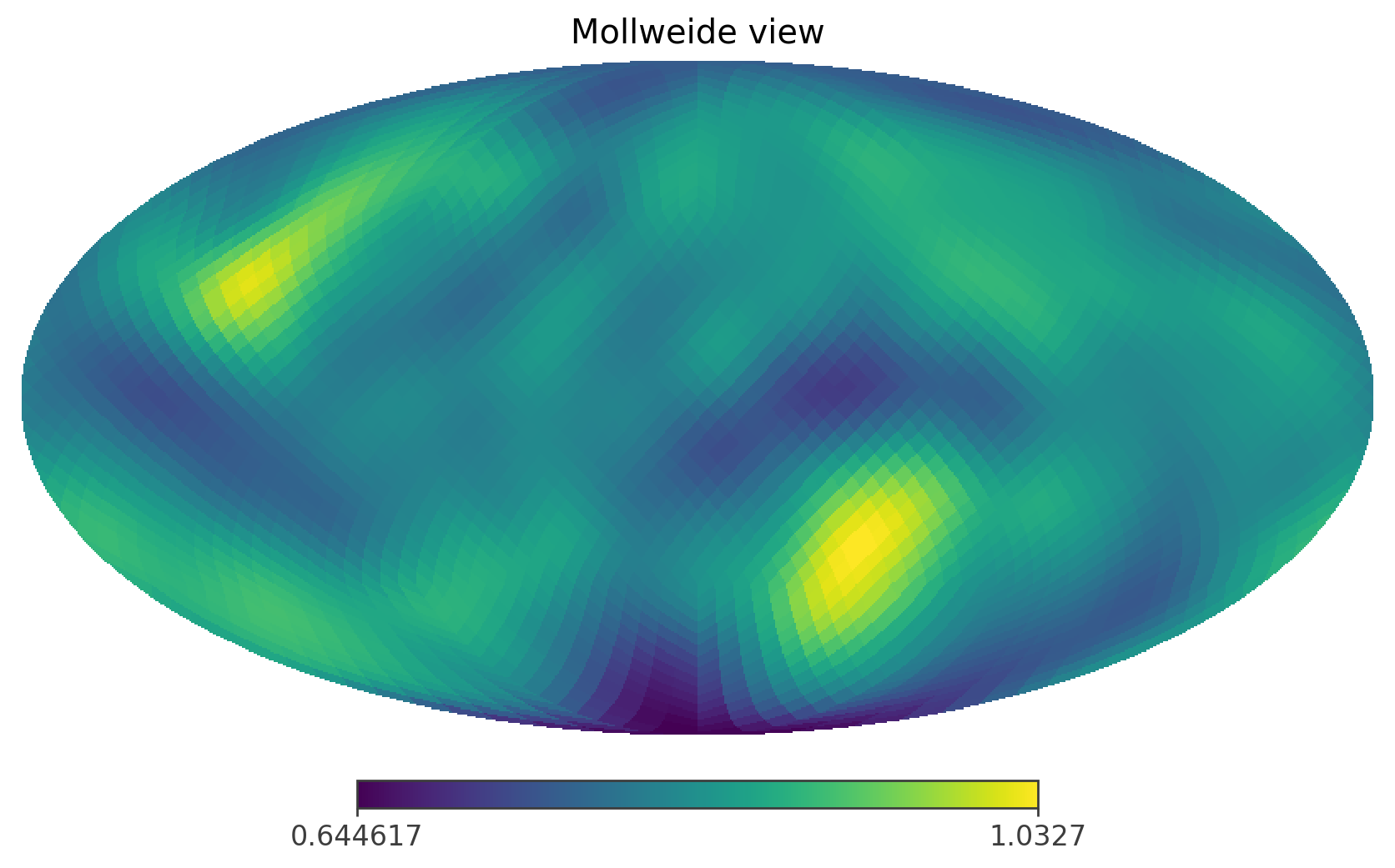
../../../_images/tutorials_background_estimation_line_background_line_background_estimation_example_notebook_49_1.png

As an future idea, applying the smoothing to the background model would be useful to mitigate the Poisson fluctutation in the backgroud model. Note that the smoothing also loses high-frequency information, so there should be optimized in some ways.

[53]:

sliced_bkg_map = bkg_model_histogram[0,0,25]

hp.mollview(sliced_bkg_map)

sliced_smoothed_bkg_map = hp.smoothing(sliced_bkg_map, fwhm = (20.0 * u.deg).to('rad').value)

hp.mollview(sliced_smoothed_bkg_map)

../../../_images/tutorials_background_estimation_line_background_line_background_estimation_example_notebook_51_0.png

../../../_images/tutorials_background_estimation_line_background_line_background_estimation_example_notebook_51_1.png

[ ]: